Basic FEM

Download this page as a Matlab LiveScript

Table of contents

Bi-linear element quadrature

Compute $\textrm{area}\left(K\right)=\int_K^{\;} dA$ for the quadrilateral element given by the coordinates below, use Gaussian quadrature to integrate!

P = [0 0 
     1 0
     0.5 0.6
     0 1];

Solution:

figure
patch(P(:,1),P(:,2),'w','FaceColor','w'); hold on
plot(P(:,1),P(:,2),'ok','MarkerFaceColor','k','MarkerSize',8,'DisplayName','Nodes')
xlabel('x')
ylabel('y')
np = size(P,1);
xm = mean(P,1);
Tp = P+(xm-P)*0.2;
text(Tp(:,1),Tp(:,2),cellstr(num2str((1:np)')),'FontSize',14)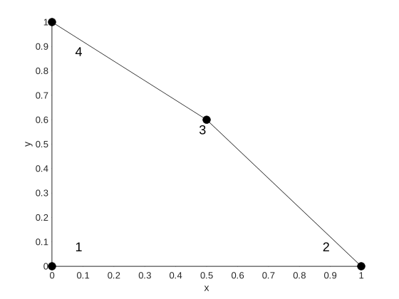

Using simple polygon area computation we can compute the area of this polygon.

area_geom = polyarea(P(:,1),P(:,2))

area_geom = 0.5500

The area (of any element) is given by the determinant of the Jacobian of the element integrated over the reference element.

We need the Jacobian

using the basis functions for the bi-linear element

phi_n = @(xi,eta)[(eta-1.0).*(xi-1.0),-xi.*(eta-1.0),eta.*xi,-eta.*(xi-1.0)];

syms xi eta
phi(xi,eta) = sym(phi_n)

The derivatives of the basis functions.

Bhat = [diff(phi,xi)
        diff(phi,eta)]

J = Bhat*P

detJ = det(J)

area = int( int( detJ ,eta,0,1),xi,0,1 )

vpa(area)

Ok, above we used symbolic integration, but we need to use Gauss quadrature to integrate $\det \left(\mathit{\bm{J} }\right)$, we can see that the function is linear in $\xi$ and $\eta$ so one-point Gauss is sufficient to integrate it exactly!

Recall

$\int_{\hat{K} }^{\;} f\left(\xi, \eta \right) d\hat{K} =\sum_i^n f\left(\xi_i ,\eta_i \right)w_i$ where the points are given in the Gauss quadrature table and $d\hat K$ is the size (area) of the reference element.

we will use $\xi =\frac{1}{2}$ and $\eta =\frac{1}{2}$ with $w_i =1$

xi = 1/2; eta = 1/2; w = 1;

area = vpa(subs(detJ))

Second order triangle quadrature

The strength of the Gaussian quadrature really shines when it comes to computing the area of curved elements. Remember, Gauss quadrature integrates these elements exactly!

Compute the area of this second order triangle with the nodal coordinates in

P = [0, 0.1
     1 0
     0 1
     0.5 -0.1
     0.5 0.6
     -0.1 0.5]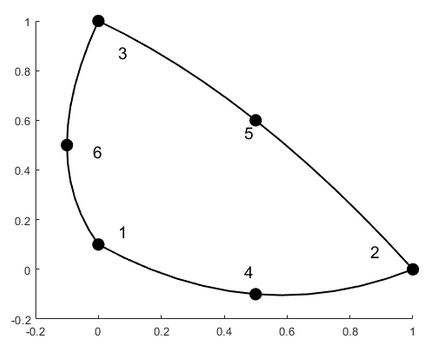

phi_n = @(xi,eta)[eta.*-3.0-xi.*3.0+eta.^2.*2.0+xi.^2.*2.0+eta.^2.*xi.^2.*1.6e1+1.0,xi.*(xi.*2.0-1.0),eta.*(eta.*2.0-1.0),xi.*(xi+eta.^2.*xi.*4.0-1.0).*-4.0,eta.^2.*xi.^2.*1.6e1,eta.*(eta+eta.*xi.^2.*4.0-1.0).*-4.0];

phi = sym(phi_n);

syms xi eta
Bhat = [diff(phi,xi)
        diff(phi,eta)];

J = Bhat*P;

detJ = det(J)

Now we compute the integral of the above expression using a second order Gauss rule since the highest polynomial term is 3.

gp = [0.5, 0
       0.5, 0.5
       0, 0.5];
gw = 1/3*[1;1;1];

The area of the reference triangle is $d \hat K = 1/2$, then we use the sum: $I = \sum_{i=1}^{n=3}\mathrm{det} \bm J (\xi_i,\eta_i) w_i d \hat K$

dk_hat = 1/2;
I = 0;
for i = 1:3
    xi = gp(i,1);
    eta = gp(i,2);
    w = gw(i);
    I = I + subs(detJ)*w*dk_hat
end

vpa(I)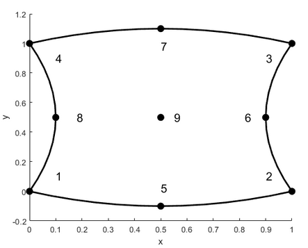

Bi-quadratic element quadrature

with nodes in

P = [0 0
     1 0
     1 1
     0 1
     0.5 -0.1
     0.9 0.5
     0.5 1.1
     0.1 0.5
     0.5 0.5];

Use Gaussian quadrature rules to integrate the area.

Use the code below to get the Gauss points and weights for the quadrilateral element:

order = 2; %Select the Gauss order here
[GP,GW] = GaussQuadrilateral(order);

We see that the area is supposed to be 1 due to symmetry.

phi = @(xi,eta)[(eta.*-3.0+eta.^2.*2.0+1.0).*(xi.*-3.0+xi.^2.*2.0+1.0),xi.*(xi.*2.0-1.0).*(eta.*-3.0+eta.^2.*2.0+1.0),eta.*xi.*(eta.*2.0-1.0).*(xi.*2.0-1.0),eta.*(eta.*2.0-1.0).*(xi.*-3.0+xi.^2.*2.0+1.0),xi.*(xi-1.0).*(eta.*-3.0+eta.^2.*2.0+1.0).*-4.0,eta.*xi.*(xi.*2.0-1.0).*(eta-1.0).*-4.0,eta.*xi.*(eta.*2.0-1.0).*(xi-1.0).*-4.0,eta.*(eta-1.0).*(xi.*-3.0+xi.^2.*2.0+1.0).*-4.0,eta.*xi.*(eta-1.0).*(xi-1.0).*1.6e1];
phi = sym(phi);
 
syms xi eta
Bhat = [diff(phi,xi)
        diff(phi,eta)];
J = Bhat*P;
detJ = det(J)

Here we evaluate the expression numerically:

detJ = matlabFunction(detJ)

detJ = 
    @(eta,xi)eta.*(-3.6e+1./2.5e+1)+xi.*(4.0./2.5e+1)+eta.*xi.*(4.8e+1./2.5e+1)-eta.*xi.^2.*(4.8e+1./2.5e+1)-eta.^2.*xi.*(4.8e+1./2.5e+1)+eta.^2.*(3.6e+1./2.5e+1)-xi.^2.*(4.0./2.5e+1)+eta.^2.*xi.^2.*(4.8e+1./2.5e+1)+2.9e+1./2.5e+1

area = detJ(GP(:,2),GP(:,1)).'*GW

area = 1.0000

function [GP,GW] = GaussQuadrilateral(order)
%GaussQuadrilateral Gauss integration scheme for quadrilateral 2D element
%   [x,y] in [0,1]

[gp,gw] = gauss(order,0,1);

[GPx,GPy] = meshgrid(gp,gp);
[Gw1,Gw2] = meshgrid(gw,gw);
GW = [Gw1(:), Gw2(:)];
GW = prod(GW,2);
GP = [GPx(:), GPy(:)];

end


function [x, w, A] = gauss(n, a, b)
%------------------------------------------------------------------------------
% gauss.m
%------------------------------------------------------------------------------
%
% Purpose:
%
% Generates abscissas and weights on I = [ a, b ] (for Gaussian quadrature).
%
%
% Syntax:
%
% [x, w, A] = gauss(n, a, b);
%
%
% Input:
%
% n    integer    Number of quadrature points.
% a    real       Left endpoint of interval.
% b    real       Right endpoint of interval.
%
%
% Output:
%
% x    real       Quadrature points.
% w    real       Weigths.
% A    real       Area of domain.
%------------------------------------------------------------------------------
% 3-term recurrence coefficients:
n = 1:(n - 1);
beta = 1 ./ sqrt(4 - 1 ./ (n .* n));
% Jacobi matrix:
J = diag(beta, 1) + diag(beta, -1); 
% Eigenvalue decomposition:
%
% e-values are used for abscissas, whereas e-vectors determine weights.
%
[V, D] = eig(J);
x = diag(D);
% Size of domain:
A = b - a;
% Change of interval:
%
% Initally we have I0 = [ -1, 1 ]; now one gets I = [ a, b ] instead.
%
% The abscissas are Legendre points.
%
if ~(a == -1 && b == 1)
  x = 0.5 * A * x + 0.5 * (b + a);
end
% Weigths:
w = V(1, :) .* V(1, :);
end